Exercise 3: DP reformulations and introduction to Control

Note

• The exercises material is divided into general information (found on this page) and the actual exercise instructions. You can download this weeks exercise instructions from here:

  • 02465ex3_Python.pdf

• You are encouraged to prepare the homework problems 1, 2 (indicated by a hand in the PDF file) at home and present your solution during the exercise session.

• To get the newest version of the course material, please see Making sure your files are up to date

This section will begin our investigation of control theory. In control theory, the time \(t\) is a continuous variable, and this will place additional requirements on the course software than the discrete-time case we have seen up to now.

To manage this complexity, the code you need to implement in order to build or test a control environment has been kept as simple as possible, and in a format that matches what you have seen so far. In other words, when you implement a new control problem, you only need to write a single class (ControlModel), and let other code deal with the tedious issues of simulation and discretization.

In this week we will only focus on defining the environment, and then next week, we will introduce some additional helper classes that will prove very helpful for building visualizations and making experiments, but which are not necessary to implement a control problem.

When we define a control environment we need to specify 3 things:

The simple bounds

These provide restrictions on e.g. the possible values of the states and actions, i.e. \(\mathbf{x}_\text{low} \leq \mathbf{x} \leq \mathbf{x}_\text{high}\) (see (Herlau [Her24], Section 10.2))

The dynamics

This is simply the differential equation \(\mathbf{f}\) defined in (Herlau [Her24], Section 10.1)

\[\frac{ dx(t)}{dt} = f(x(t), u(t), t)\]

The cost function

This measures how good (or bad) a control trajectory is and is defined in (Herlau [Her24], eq. (10.12)), and is defined in the class SymbolicQRCost.

These quantities are specified in the class ControlModel, and parallel what you saw in the dynamical programming model.

Specifying a model

Specifying a model is easiest done by creating a class that inherits from ControlModel and implementing the bounds, dynamics and cost. As an example, we will consider a simple version of the Pendulum model. Recall that in this environment the state is 2-dimensional, corresponding to the pendulum angle and angular velocity:

\[\begin{split}\mathbf{x} = \begin{bmatrix} \theta \\ \dot \theta \end{bmatrix}\end{split}\]

and the control is 1-dimensional corresponding to a torque. The implementation of this model looks as follows:

# basic_pendulum.py
class BasicPendulumModel(ControlModel): 
    def sym_f(self, x, u, t=None):
        g = 9.82
        l = 1
        m = 2
        theta_dot = x[1]  # Parameterization: x = [theta, theta']
        theta_dot_dot = g / l * sym.sin(x[0]) + 1 / (m * l ** 2) * u[0]
        return [theta_dot, theta_dot_dot]

    def get_cost(self) -> SymbolicQRCost:
        return SymbolicQRCost(Q=np.eye(2), R=np.eye(1))

    def u_bound(self) -> Box:
        return Box(np.asarray([-10]), np.asarray([10]))

    def x0_bound(self) -> Box:
        return Box(np.asarray( [np.pi, 0] ), np.asarray( [np.pi, 0])) 

This is a fairly long listing, so lets go over each of the three components:

Tip

You are not required to specify bounds. If you do not specify bounds the system will default to no restrictions on all variables except for \(t_0\) which is set to \(t_0 = 0\).

The dynamics:

The dynamics is specified in the function sym_f as a function that accepts two input arguments, x and u , and should return a new list where each element corresponds to the corresponding element in \(\mathbf{f}\). The output is therefore two-dimensional.

The Cost:

The cost is defined in the function get_cost. It should return a SymbolicQRCost. object, in this case it uses \(Q=I\) and \(R=I\).

The bounds:

There are two bounds specified. The first imposes a restriction on the controls: \(-10 \leq \mathbf{u}(t) \leq 10\) and the second that the system starts in the hangin-down position: \(\begin{bmatrix} \pi \\ 0 \end{bmatrix} \leq \mathbf{x}(t_0) \leq \begin{bmatrix} \pi \\ 0 \end{bmatrix}\). Note that the functions should return a gymnasium.spaces.Box-instance.

Once defined, you can access the bounds and the cost-matrices as follows:

>>> from irlc.ex03.basic_pendulum import BasicPendulumModel
>>> model = BasicPendulumModel()
>>> cost = model.get_cost() # Get the cost function object
>>> print("The Q-matrix is")
The Q-matrix is
>>> print(cost.Q)
[[1. 0.]
 [0. 1.]]
>>> print("The upper and lower bounds on u is", model.u_bound().low, model.u_bound().high)
The upper and lower bounds on u is [-10.] [10.]
>>> print("Unspecified bounds default to inf:", model.x_bound().low, model.x_bound().high)
Unspecified bounds default to inf: [-inf -inf] [inf inf]

Note

The dimensions of x and u are determined by the cost function. It is therefore important that you specify at least the \(Q\) and \(R\)-matries with the appropriate dimensions.

In the next week, it will turn out to be very convenient to be able to compute derivatives of the dynamics \(\mathbf{f}\). To do that effectively, we will use the library sympy. Sympy is easy to work with, but if you are unfamiliar with it there is a primer below. Once the model is defined, you can use print to get an overview of how it is defined – I recommend doing this for verification. An example:

>>> from irlc.ex03.basic_pendulum import BasicPendulumModel
>>> model = BasicPendulumModel()
>>> print(model)
<class 'irlc.ex03.basic_pendulum.BasicPendulumModel'>
==================================================
Dynamics:
--------------------
    [x0]          [                   x1]
  f([x1], [u0]) = [0.5*u0 + 9.82*sin(x0)]
Cost:
--------------------
Continuous-time cost function:
> Non-zero terms in c(x, u):
 * Q = 
[[1. 0.]
 [0. 1.]]
 * R = [[1.]]

Bounds:
--------------------
low                    variable    high
---------------------  ----------  ---------------------
[3.1415927 0.       ]  <= x0 <=    [3.1415927 0.       ]
-10.0                  <= u <=     10.0
0.0                    <= t0 <=    0.0

Simulating a policy

The model contains a build in simulation function irlc.ex03.control_model.ControlModel.simulate(). The function requires an action sequence, for which you have two choices:

• To pass a general policy function u(x,t) which will then be used to compute actions

• To pass a constant (numpy) value of the action sequence \(u_0\), in which case the policy is assumed constant \(u(x,t) = u_0\)

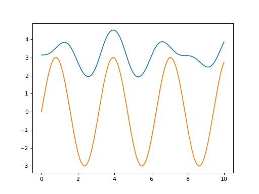
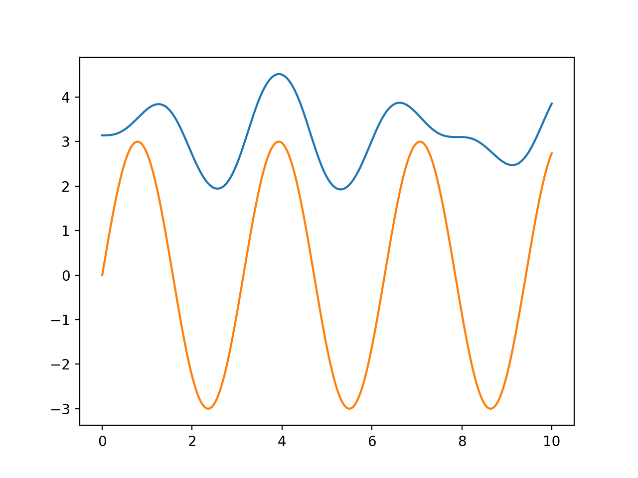
Click on the Source code link to see how the following example simulate the policy \(u(x,t) = 3 \sin(2t)\) and plot the outcome:

(Source code, png, hires.png, pdf)

Defining bounds

The simple bounds serve a simple purposes, namely to tell us what values the states and actions can possibly take (see (Herlau [Her24], Section 10.2) for a full list of bounds). The following table provides an overview and the last column is their default value. See also gymnasium.spaces.Box.

Available bounds

Bound	Function	Default value
Bound on states: \(\mathbf{x}^\text{low} \leq \mathbf{x}(t) \leq \mathbf{x}^\text{high}\)	x_bound()	# control_model.py def x_bound(self) -> Box: r"""The bound on all other states :math:`\mathbf{x}(t)`. :return: An appropriate gymnasium Box instance. """ return Box(-np.inf, np.inf, shape=(self.state_size,))
Bound on actions: \(\mathbf{u}^\text{low} \leq \mathbf{u}(t) \leq \mathbf{u}^\text{high}\)	u_bound()	# control_model.py def u_bound(self) -> Box: r"""The bound on the terminal state :math:`\mathbf{u}(t)`. :return: An appropriate gymnasium Box instance. """ return Box(-np.inf, np.inf, shape=(self.action_size,))
Bound on start time: \(\mathbf{t_F}^\text{low} \leq t_F \leq \mathbf{t_F}^\text{high}\)	tF_bound()	# control_model.py def tF_bound(self) -> Box: r"""The bound on the final time :math:`\mathbf{t}_F`, i.e. when the environment terminates. :return: An appropriate gymnasium Box instance. """ return Box(-np.inf, np.inf, shape=(1,))
Bound on end time: \(\mathbf{t_0}^\text{low} \leq t_0 \leq \mathbf{t_0}^\text{high}\)	t0_bound()	# control_model.py def t0_bound(self) -> Box: r"""The bound on the initial time :math:`\mathbf{t}_0`. I have included this bound for completeness: In practice, there is no reason why you should change it from the default bound is ``Box(0, 0, shape=(1,))``, i.e. :math:`\mathbf{t}_0 = 0`. :return: An appropriate gymnasium Box instance. """ return Box(0, 0, shape=(1,))
Bound on initial state: \(\mathbf{x_0}^\text{low} \leq \mathbf{x}(t_0) \leq \mathbf{x_0}^\text{high}\)	x0_bound()	# control_model.py def x0_bound(self) -> Box: r"""The bound on the initial state :math:`\mathbf{x}_0`. The default bound is ``Box(0, 0, shape=(self.state_size,))``, i.e. :math:`\mathbf{x}_0 = 0`. :return: An appropriate gymnasium Box instance. """ return Box(0, 0, shape=(self.state_size,))
Bound on terminal state: \(\mathbf{x_F}^\text{low} \leq \mathbf{x}(t_F) \leq \mathbf{x_F}^\text{high}\)	xF_bound()	# control_model.py def xF_bound(self) -> Box: r"""The bound on the terminal state :math:`\mathbf{x}_F`. :return: An appropriate gymnasium Box instance. """ return Box(-np.inf, np.inf, shape=(self.state_size,))

Warning

Bounds are mostly relevant for direct control methods. I recommend that you don’t specify the bounds unless you specifically need them.

According to the default values the system has no restrictions except for the initial state which defaults to the equality constraint \(\mathbf{x}(t_0) = \mathbf{0}\) and the initial time \(t_0 = 0\). When the initial state is set using an equality constraint, you can access the initial state as follows:

>>> from irlc.ex03.basic_pendulum import BasicPendulumModel
>>> model = BasicPendulumModel()
>>> print("The initial state is x0 =", model.x0_bound().low)
The initial state is x0 = [3.1415927 0.       ]

States and actions

States and actions are represented as vectors. You can get the dimension \(n\) of the state \(x\) and dimension \(d\) of the actions \(u\) as follows:

>>> from irlc.ex04.model_pendulum import PendulumModel
>>> model = PendulumModel()
>>> print("n =", model.state_size, "and d =", model.action_size)
n = 2 and d = 1

Computing the dynamics

The dynamics is specified as a symbolic expression f() is specified as a sympy object (Herlau [Her24], Section 10.1). However, the ControlModel will automatically generate a numpy equivalent which is what you will use in the exercises. In other words, you can evaluate it in two ways:

As a numpy expression:

Use model.f. An example:

>>> from irlc.ex04.model_pendulum import PendulumModel
>>> model = PendulumModel()
>>> x = model.x0_bound().low # Get the initial state
>>> u = [1]                    # A torque of unit
>>> model.f(x, u, t=0) # Evaluate the dynamics
array([0.        , 1.24999914])

As a sympy expression:

Use model.sym_f. In order to call this function, we must create symbolic variables x, u and t of the right dimensions:

>>> from irlc.ex04.model_pendulum import PendulumModel
>>> import sympy as sym
>>> model = PendulumModel()
>>> x = sym.symbols('x0:2')  # Generates a list with 2 symbolic variables [x_0, x_1]
>>> u = sym.symbols('u0:1')  # Create a list of one symbolic variable [u0]
>>> t = sym.symbols('t')     # the time variable (required but not used)
>>> model.sym_f(x, u, t)     # Returns a symbolic expression corresponding to f(x, u)cd
[x1, 1.25*u0 + 9.82*sin(x0)]

Tip

Note that we represent vectors as lists of symbolic expressions. The function will therefore return a length 2 list with 2 symbolic expressions, each corresponding to a coordinate of \(\dot f\).

The cost-function

The model must also specify a cost-function (Herlau [Her24], Subsection 10.3.1). I have chosen to de-emphasize the cost-function in this course since the treatment is similar (but conceptually simpler) than the implementation of the dynamics, but the implementation tends to be more messy since the cost function will typically involve many terms. For now, simply note that you can access the cost function and print the cost matrices, and the value of the cost function, as follows:

>>> from irlc.ex04.model_pendulum import PendulumModel
>>> model = PendulumModel()
>>> cost = model.get_cost() # This function returns a cost-object.
>>> cost.Q # Get access to a single cost matrix.
array([[1., 0.],
       [0., 1.]])
>>> print(cost)   # Print the cost function in a nicer format.
Continuous-time cost function:
> Non-zero terms in c(x, u):
 * Q = 
[[1. 0.]
 [0. 1.]]
 * R = [[1.]]

Background: Symbolic expressions and sympy

Sympy is a symbolic math library for python. You can think about it as a greatly simplified version of pytorch, or a python-version of Maple. Mat1 will in fact replace Maple with sympy in 2023. Using sympy involves this procedure:

• Specify a sympy expression using the sympy python-library

• Perform operations on the expression, such as substitutions, algebraic operations or computation of derivatives

• Transform the sympy expression into a python function. This function will take numerical values as input and return numerical values.

Let’s look at an example. This code computes the derivative of \(x^3\):

>>> import sympy as sym
>>> x = sym.symbols("x") # Create a sympy expression. Compare this to a torch.Tensor
>>> y = x ** 3           # Note that y is also a sympy expression.
>>> print(y)
x**3
>>> dydx = sym.diff(y, x) # Compute the derivative; this too is a sympy expression.
>>> print(dydx)
3*x**2

The final expression is still a sympy object. To turn it into a numpy expression we would do the following:

>>> import sympy as sym
>>> x = sym.symbols("x")                        # Create a sympy expression. Compare this to a torch.Tensor
>>> dydx = sym.diff(x**3, x)                    # Compute the derivative; this too is a sympy expression.
>>> y_numpy = sym.lambdify(x, dydx)             # y_numpy is now a numpy function.
>>> value = y_numpy(2)                          # Note: This function takes numbers as input and returns numbers.
>>> print("dx^3/dx evaluated in x=2 is", value)
dx^3/dx evaluated in x=2 is 12

You might notice that the function sym.lambdify returns a function. This is called a higher-order function if you are curious. The bottom line is that the above recipe (starting from sympy variables, somehow turning them into another sympy expression, and finally ending with sym.lambdify) will be representative of how we use sympy throughout this course.

Classes and functions

class irlc.ex03.control_model.ControlModel

Represents the continious time model of a control environment.

See (Her24, Section 13.2) for a top-level description.

The model represents the physical system we are simulating and can be considered a control-equivalent of the irlc.ex02.dp_model.DPModel. The class must keep track of the following:

\[\frac{dx}{dt} = f(x, u, t)\]

And the cost-function which is defined as an integral

\[c_F(t_0, t_F, x(t_0), x(t_F)) + \int_{t_0}^{t_F} c(t, x, u) dt\]

as well as constraints and boundary conditions on \(x\), \(u\) and the initial conditions state \(x(t_0)\). this course, the cost function will always be quadratic, and can be accessed as model.get_cost.

If you want to implement your own model, the best approach is to start with an existing model and modify it for your needs. The overall idea is that you implement the dynamics,``sym_f``, and the cost function get_cost, and optionally define bounds as needed.

__init__()

The cost must be an instance of irlc.ex04.cost_continuous.SymbolicQRCost. Bounds is a dictionary but otherwise optional; the model should give it a default value.

Parameters:

• cost – A quadratic cost function

• bounds (dict) – A dictionary of boundary constraints.

x0_bound()

The bound on the initial state \(\mathbf{x}_0\).

The default bound is Box(0, 0, shape=(self.state_size,)), i.e. \(\mathbf{x}_0 = 0\).

Return type:

Box

Returns:

An appropriate gymnasium Box instance.

xF_bound()

The bound on the terminal state \(\mathbf{x}_F\).

Return type:

Box

Returns:

An appropriate gymnasium Box instance.

x_bound()

The bound on all other states \(\mathbf{x}(t)\).

Return type:

Box

Returns:

An appropriate gymnasium Box instance.

u_bound()

The bound on the terminal state \(\mathbf{u}(t)\).

Return type:

Box

Returns:

An appropriate gymnasium Box instance.

t0_bound()

The bound on the initial time \(\mathbf{t}_0\).

I have included this bound for completeness: In practice, there is no reason why you should change it from the default bound is Box(0, 0, shape=(1,)), i.e. \(\mathbf{t}_0 = 0\).

Return type:

Box

Returns:

An appropriate gymnasium Box instance.

tF_bound()

The bound on the final time \(\mathbf{t}_F\), i.e. when the environment terminates.

Return type:

Box

Returns:

An appropriate gymnasium Box instance.

sym_f(x, u, t=None)

The symbolic (sympy) version of the dynamics \(f(x, u, t)\). This is the main place where you specify the dynamics when you build a new model. you should look at concrete implementations of models for specifics.

Parameters:

• x – A list of symbolic expressions ['x0', 'x1', ..] corresponding to \(x\)

• u – A list of symbolic expressions ['u0', 'u1', ..] corresponding to \(u\)

• t – A single symbolic expression corresponding to the time \(t\) (seconds)

Returns:

A list of symbolic expressions [f0, f1, ...] of the same length as x where each element is a coordinate of \(f\)

f(x, u, t=0)

Evaluate the dynamics.

This function will evaluate the dynamics. In other words, it will evaluate \(\mathbf{f}\) in the following expression:

\[\dot{\mathbf{x}} = \mathbf{f}(\mathbf{x}, \mathbf{u}, t)\]

Parameters:

• x – A numpy ndarray corresponding to the state

• u – A numpy ndarray corresponding to the control

• t – A float corresponding to the time.

Return type:

ndarray

Returns:

The time derivative of the state, \(\mathbf{x}(t)\).

simulate(x0, u_fun, t0, tF, N_steps=1000, method='rk4')

Used to simulate the effect of a policy on the model. By default, it uses Runge-Kutta 4 (RK4) with a fine discretization – this is slow, but in nearly all cases exact. See (Her24, Algorithm 18) for more information.

The input argument u_fun should be a function which returns a list or tuple with same dimension as model.action_space, \(d\).

Parameters:

• x0 – The initial state of the simulation. Must be a list of floats of same dimension as env.observation_space, \(n\).

• u_fun – Can be either: - Either a policy function that can be called as u_fun(x, t) and returns an action u in the action_space - A single action (i.e. a list of floats of same length as the action space). The model will be simulated with a constant action in this case.

• t0 (float) – Starting time \(t_0\)

• tF (float) – Stopping time \(t_F\); the model will be simulated for \(t_F - t_0\) seconds

• N_steps (int) – Steps \(N\) in the RK4 simulation

• method (str) – Simulation method. Either 'rk4' (default) or 'euler'

Returns:

• xs - A numpy ndarray of dimension \((N+1)\times n\) containing the observations \(x\)

• us - A numpy ndarray of dimension \((N+1)\times d\) containing the actions \(u\)

• ts - A numpy ndarray of dimension \((N+1)\) containing the corresponding times \(t\) (seconds)

property state_size

This field represents the dimensionality of the state-vector \(n\). Use it as model.state_size :return: Dimensionality of the state vector \(x\)

property action_size

This field represents the dimensionality of the action-vector \(d\). Use it as model.action_size :return: Dimensionality of the action vector \(u\)

render(x, render_mode='human')

Responsible for rendering the state. You don’t have to worry about this function.

Parameters:

• x – State to render

• render_mode (str) – Rendering mode. Select "human" for a visualization.

Returns:

Either none or a ndarray for plotting.

phi_x(x)

Coordinate transformation of the state when the model is discretized.

This function specifies the coordinate transformation \(x_k = \Phi_x(x(t_k))\) which is applied to the environment when it is discretized. It should accept a list of symbols, corresponding to \(x\), and return a new list of symbols corresponding to the (discrete) coordinates.

Parameters:

x (list) – A list of symbols [x0, x1, ..., xn] corresponding to \(\mathbf{x}(t)\)

Return type:

list

Returns:

A new list of symbols corresponding to the discrete coordinates \(\mathbf{x}_k\).

phi_x_inv(x)

Inverse of coordinate transformation for the state.

This function should specify the inverse of the coordinate transformation \(\Phi_x\), i.e. \(\Phi_x^{-1}\). In other words, it has to map from the discrete coordinates to the continuous-time coordinates: \(x(t) = \Phi_x^{-1}(x_k)\).

Parameters:

x (list) – A list of symbols [x0, x1, ..., xn] corresponding to \(\mathbf{x}_k\)

Return type:

list

Returns:

A new list of symbols corresponding to the continuous-time coordinates \(\mathbf{x}(t)\).

phi_u(u)

Coordinate transformation of the action when the model is discretized.

This function specifies the coordinate transformation \(x_k = \Phi_x(x(t_k))\) which is applied to the environment when it is discretized. It should accept a list of symbols, corresponding to \(x\), and return a new list of symbols corresponding to the (discrete) coordinates.

Parameters:

x – A list of symbols [x0, x1, ..., xn] corresponding to \(\mathbf{x}(t)\)

Return type:

list

Returns:

A new list of symbols corresponding to the discrete coordinates \(\mathbf{x}_k\).

phi_u_inv(u)

Inverse of coordinate transformation for the action.

This function should specify the inverse of the coordinate transformation \(\Phi_u\), i.e. \(\Phi_u^{-1}\). In other words, it has to map from the discrete coordinates to the continuous-time coordinates: \(u(t) = \Phi_u^{-1}(u_k)\).

Parameters:

x – A list of symbols [u0, u1, ..., ud] corresponding to \(\mathbf{u}_k\)

Return type:

list

Returns:

A new list of symbols corresponding to the continuous-time coordinates \(\mathbf{u}(t)\).

class irlc.ex03.control_cost.SymbolicQRCost(Q, R, q=None, qc=None, r=None, H=None, QN=None, qN=None, qcN=None)

This class represents the cost function for a continuous-time model. In the simulations, we are going to assume that the cost function takes the form:

\[\int_{t_0}^{t_F} c(x(t), u(t)) dt + c_F(x_F)\]

And this class will specifically implement the two functions \(c\) and \(c_F\). They will be assumed to have the quadratic form:

\[\begin{split}c(x, u) & = \frac{1}{2} x^T Q x + \frac{1}{2} u^T R u + u^T H x + q^T x + r^T u + q_0, \\ c_F(x_F) & = \frac{1}{2} x_F^T Q_F x_F + q_F^T x_F + q_{0,F}.\end{split}\]

So what all of this boils down to is that the class just need to store a bunch of matrices and vectors.

You can add and scale cost-functions

A slightly smart thing about the cost functions are that you can add and scale them. The following provides an example:

>>> from irlc.ex03.control_cost import SymbolicQRCost
>>> import numpy as np
>>> cost1 = SymbolicQRCost(np.eye(2), np.zeros(1) ) # Set Q = I, R = 0
>>> cost2 = SymbolicQRCost(np.ones((2,2)), np.zeros(1) ) # Set Q = 2x2 matrices of 1's, R = 0
>>> print(cost1.Q) # Will be the identity matrix.
[[1. 0.]
 [0. 1.]]
>>> cost = cost1 * 3 +  cost2 * 2
>>> print(cost.Q) # Will be 3 x I + 2
[[5. 2.]
 [2. 5.]]

__init__(Q, R, q=None, qc=None, r=None, H=None, QN=None, qN=None, qcN=None)

The constructor can be used to manually create a cost function. You will rarely want to call the constructor directly but instead use the helper methods (see class documentation). What the class basically does is that it stores the input parameters as fields. In other words, you can access the quadratic term of the cost function, \(\frac{1}{2}x^T Q x\), as cost.Q.

Parameters:

• Q – The matrix \(Q\)

• R – The matrix \(R\)

• q – The vector \(q\)

• qc – The constant \(q_0\)

• r – The vector \(r\)

• H – The matrix \(H\)

• QN – The terminal cost matrix \(Q_N\)

• qN – The terminal cost vector \(q_N\)

• qcN – The terminal cost constant \(q_{0,N}\)

classmethod zero(state_size, action_size)

Creates an all-zero cost function, i.e. all terms \(Q\), \(R\) are set to zer0.

>>> from irlc.ex03.control_cost import SymbolicQRCost
>>> cost = SymbolicQRCost.zero(2, 1)
>>> cost.Q # 2x2 zero matrix
array([[0., 0.],
       [0., 0.]])
>>> cost.R # 1x1 zero matrix.
array([[0.]])

Parameters:

• state_size – Dimension of the state vector \(n\)

• action_size – Dimension of the action vector \(d\)

Returns:

A SymbolicQRCost with all zero terms.

sym_c(x, u, t=None)

Evaluate the (instantaneous) part of the function \(c(x,u, t)\). An example:

>>> from irlc.ex03.control_cost import SymbolicQRCost
>>> import numpy as np
>>> cost = SymbolicQRCost(np.eye(2), np.eye(1)) # Set Q = I, R = 0
>>> cost.sym_c(x = np.asarray([1,2]), u=np.asarray([0])) # should return 0.5 * x^T Q x = 0.5 * (1 + 4)
2.50000000000000

Parameters:

• x – The state \(x(t)\)

• u – The action \(u(t)\)

• t – The current time step \(t\) (this will be ignored)

Returns:

A sympy symbolic expression corresponding to the instantaneous cost.

sym_cf(t0, tF, x0, xF)

Evaluate the terminal (constant) term in the cost function \(c_F(t_0, t_F, x_0, x_F)\). An example:

>>> from irlc.ex03.control_cost import SymbolicQRCost
>>> import numpy as np
>>> cost = SymbolicQRCost(np.eye(2), np.zeros(1), QN=np.eye(2)) # Set Q = I, R = 0
>>> cost.sym_cf(0, 0, 0, xF=2*np.ones((2,))) # should return 0.5 * xF^T * xF = 0.5 * 8
4.00000000000000

Parameters:

• t0 – Starting time \(t_0\) (not used)

• tF – Stopping time \(t_F\) (not used)

• x0 – Initial state \(x_0\) (not used)

• xF – Termi lanstate \(x_F\) (this one is used)

Returns:

A sympy symbolic expression corresponding to the terminal cost.

discretize(dt)

Discretize the cost function so it is suitable for a discrete control problem. See (Her24, Subsection 13.1.5) for more information.

Parameters:

dt – The discretization time step \(\Delta\)

Returns:

An DiscreteQRCost instance corresponding to a discretized version of this cost function.

goal_seeking_terminal_cost(xF_target, QF=None)

Create a cost function which is minimal when the terminal state \(x_F\) is equal to a goal state \(x_F^*\). Concretely, it will return a cost function of the form

\[c_F(x_F) = \frac{1}{2} (x_F^* - x_F)^\top Q_F (x_F^* - x_F)\]

>>> from irlc.ex03.control_cost import SymbolicQRCost
>>> import numpy as np
>>> cost = SymbolicQRCost.zero(2, 1)
>>> cost += cost.goal_seeking_terminal_cost(xF_target=np.ones((2,)))
>>> print(cost.qN)
[-1. -1.]
>>> print(cost)
Continuous-time cost function:
> Non-zero terms in c_F(x):
 * QN = 
[[1. 0.]
 [0. 1.]]
 * qN = [-1. -1.]
 * qcN = 1.0

Parameters:

• xF_target – Target state \(x_F^*\)

• QF – Cost matrix \(Q_F\)

Returns:

A SymbolicQRCost object corresponding to the goal-seeking cost function

goal_seeking_cost(x_target, Q=None)

Create a cost function which is minimal when the state \(x\) is equal to a goal state \(x^*\). Concretely, it will return a cost function of the form

\[c(x, u) = \frac{1}{2} (x^* - x)^\top Q (x^* - x)\]

>>> from irlc.ex03.control_cost import SymbolicQRCost
>>> import numpy as np
>>> cost = SymbolicQRCost.zero(2, 1)
>>> cost += cost.goal_seeking_cost(x_target=np.ones((2,)))
>>> print(cost.q)
[-1. -1.]
>>> print(cost)
Continuous-time cost function:
> Non-zero terms in c(x, u):
 * Q = 
[[1. 0.]
 [0. 1.]]
 * q = [-1. -1.]
 * qc = 1.0

Parameters:

• x_target – Target state \(x^*\)

• Q – Cost matrix \(Q\)

Returns:

A SymbolicQRCost object corresponding to the goal-seeking cost function

Solutions to selected exercises

Problem 3.5: Exact evaluation of DP

Exercise 3.6: Toy 2d control

Solution to problem 1

Part a: First insert and integrate to get

\[\dot x(t) = e^{-x(t)} u(t) = e^{-x(t)} 2t\]

A standard strategy is to isolate the function we wish to solve for. This gives:

\[2t = \dot x(t) e^{x(t)} = \frac{d}{dt} e^{x(t)}\]

Integrating to to get:

\[t^2 + k = e^{x(t)}\]

The boundary condition gives \(x(t) = \log(t^2 + e)\)

Part b: Inserting into the cost function and integrate gives:

\[\int_{0}^{t_F} e^{x(t)} dt = \int_{0}^{t_F} (e + t^2) = t_F e + \frac{1}{3}t_F^3\]

Comment: The purpose of this exercise is both to familiarize you with the notation, and more fundamentally to simply observe that for a given choice of actions, it is in principle possible to determine the cost-function exactly. From here on we could in principle try to optimize (solve) for the optimal action sequence. For instance, you can try to re-do the problem using a sequence \(u(t) = at\) and try to determine the optimal value of \(a\).

Solution to problem 4: Pen-and-paper DP

Part a: This expression is relevant because \(J_k(x_k) = \min_u Q(x_k, u)\) – and it was in fact the expression we computed when we implemented when we implemented the DP algorithm last week. Looking ahead, an expression \(Q\) (with a slightly adapted definition) will play a key role in reinforcement learning.

Part b: If we insert the expressions for \(g_k\) and \(f_k\) we get:

\[\begin{split}Q(x, u) & = \mathbb{E}[(x + w - u)^2 + \log 2 e^{(x+w-u)^2} ] \\ & = \log 2 + 2\mathbb{E}[ (x + w - u)^2]\end{split}\]

When dealing with expectations, a good strategy is to expand and use linearity. If we expand the square we get:

\[\begin{split}Q(x, u) & = \log 2 + 2\mathbb{E}[ (x - u)^2 + w^2 - 2w(x-u)] \\ & = \log 2 + 2 (x - u)^2 + 2\mathbb{E}[w^2] - 4(x-u) \mathbb{E}[w]\end{split}\]

Then simply recall that \(\mathbb{E}[w] = 0\) and \(\mathbb{E}[w^2] = 1\) since \(w\) follows a standard normal distribution (mean 0 and unit variance) and we get:

\[Q(x, u) = \log 2 + 2 + 2 (x - u)^2\]

Part c+d: The optimal policy is found by minimizing over actions – clearly this occurs when \(x = u\) so:

\[\mu_{N-1}(x_{N-1}) = \arg\min_{u} Q(x_k, u) = x_k\]

and

\[J_{N-1}(x_{N-1}) = \min_{u} Q(x_k, u) = \log 2 + 2\]

Part f: The only thing that would change is that \(\mathbb{E}[w^2] = \sigma^2\). Therefore

\[Q_\sigma(x, u) = \log 2 + 2\sigma^2 + 2 (x - u)^2 = Q(x, u) - 2 + 2\sigma^2\]

I.e., the only change is a constant factor that does not affect the optimal policy.

This is perhaps rather strange – adding noise, regardless of how much, does not change what we should do, it just jiggles us around a bit and affects the expected cost.

Comment: We will re-do something similar to this calculation when we derive discrete LQR, but the math will be slighly more tedious. The last result, that noise does not affect the optimal policy, is mainly a consequence of the noise being symmetric around 0 – and the same lesson will carry over when we consider LQR.