Exercise 4: Discretization and PID control

Note

• The exercises material is divided into general information (found on this page) and the actual exercise instructions. You can download this weeks exercise instructions from here:

  • 02465ex4_Python.pdf

• You are encouraged to prepare the homework problems 1, 2 (indicated by a hand in the PDF file) at home and present your solution during the exercise session.

• To get the newest version of the course material, please see Making sure your files are up to date

Last week we saw how we could specify a basic control model using the irlc.ex03.control_model.ControlModel class. This model implements a continuous-time environment of the form

\[\mathbf{\dot{x}} = \mathbf{f}(\mathbf{x}, \mathbf{u}, t)\]

In this week, we will consider discretization, which is the process of turning the environment into the form:

\[\mathbf{x}_{k+1} = f_k(\mathbf{x}_k, \mathbf{u}_k) = \mathbf{x}_{k} + \Delta \mathbf{f}(\mathbf{x}_k, \mathbf{u}_k, t_k)\]

Discretization is an automatic procecure, which means that you only need to understand this part of the code from a user-perspective.

To give an overview, we end up with three classes:

The ControlModel class

This is the main class. It implements and represents everything that has to do with the continuous-time control problem. This includes:

• The differential equation

  \[\frac{ dx(t)}{dt} = f(x(t), u(t), t)\]

  which you implement as sym_f

• The cost-function

  \[g(x(t), u(t), t) = \frac{1}{2} x(t)^\top Q x(t) + \frac{1}{2} u(t)^\top R u(t) + \cdots\]

  which you implement as get_cost

The DiscreteControlModel

This class represents a discretized version of a continuous control problem. You call it with a ControlModel object and a discretization time \(\Delta\), which it will then discretize for you. It will give you:

• Specifying the (Euler) discretized dynamics: \(x_{k+1} = f_k(x_k, u_k)\) (as f())

• Ability to evaluate the discretized cost function (as as c() and as cN(), the later being the terminal cost).

• Ability to compute gradients of the dynamics using (as f_jacobian())

The ControlEnvironment

This class represents a control environment – i.e. this is the class you pass on to the train()-method, and it is an instance of the base environment class we saw in week 1-3, gymnasium.Env.

To create an environment, you simply give it a DiscreteControlModel object, and a maximum time until the environment terminates Tmax.

• It has a step and reset function as any other environment.

The bottom line of the above is that your main work will be in specifying the continuous time model, and then the discrete model and environment can be derived automatically in potentially very few lines.

Example: Creating a discrete pendulum environment

As an example, lets create a discrete version of the basic pendulum environment we saw in last week.

Starting point

Our starting point is the ControlModel object we saw last week:

# basic_pendulum.py
class BasicPendulumModel(ControlModel): 
    def sym_f(self, x, u, t=None):
        g = 9.82
        l = 1
        m = 2
        theta_dot = x[1]  # Parameterization: x = [theta, theta']
        theta_dot_dot = g / l * sym.sin(x[0]) + 1 / (m * l ** 2) * u[0]
        return [theta_dot, theta_dot_dot]

    def get_cost(self) -> SymbolicQRCost:
        return SymbolicQRCost(Q=np.eye(2), R=np.eye(1))

    def u_bound(self) -> Box:
        return Box(np.asarray([-10]), np.asarray([10]))

    def x0_bound(self) -> Box:
        return Box(np.asarray( [np.pi, 0] ), np.asarray( [np.pi, 0])) 

Discretize the control model

The following two lines will discretize the pendulum model and display information about it:

>>> from irlc.ex04.discrete_control_model import DiscreteControlModel
>>> from irlc.ex03.basic_pendulum import BasicPendulumModel
>>> model = BasicPendulumModel()
>>> discrete_pendulum = DiscreteControlModel(model, dt=0.5)  # Using a discretization time step: 0.5 seconds.
>>> print(discrete_pendulum)
<class 'irlc.ex04.discrete_control_model.DiscreteControlModel'>
==================================================
Dynamics (after discretization with Delta = 0.5):
--------------------
    [x0]          [                x0 + 0.5*x1]
  f([x1], [u0]) = [0.25*u0 + x1 + 4.91*sin(x0)]
Continuous-time dynamics:
--------------------
f_k((x0, x1), (u0,)) = [x1, 0.5*u0 + 9.82*sin(x0)]

Variable transformations:
--------------------
 * phi_x( x(t) ) -> x_k = (x0, x1)
 * phi_u( u(t) ) -> u_k = (u0,)

Cost:
--------------------
Discrete-time cost function:
> Non-zero terms in c_k(x_k, u_k):
 * Q = 
[[0.5 0. ]
 [0.  0.5]]
 * R = [[0.5]]

Computing the discrete dynamics

To compute the discrete dynamics, use irlc.ex04.discrete_control_model.DiscreteControlModel.f(). As an example:

>>> from irlc.ex04.discrete_control_model import DiscreteControlModel
>>> from irlc.ex03.basic_pendulum import BasicPendulumModel
>>> model = BasicPendulumModel()
>>> discrete_pendulum = DiscreteControlModel(model, dt=0.5)  # Using a discretization time step: 0.5 seconds.
>>> x0 = model.x0_bound().low # Get the initial state: x0 = [np.pi, 0].
>>> u0 = [0.1] # Action of u=0.1. Note that the action must be a list.
>>> x1 = discrete_pendulum.f(x0, u0)
>>> print(x1)
[3.14159274 0.02499957]
>>> print("Now, lets compute the Euler step manually to confirm")
Now, lets compute the Euler step manually to confirm
>>> x1_manual = x0 + 0.5 * model.f(x0, u0)
>>> print(x1_manual)
[3.14159274 0.02499957]

The default discretization procedure is Euler discretization which the two last lines verify.

Pendulum continued: Coordinate transformations

It is common to apply a variable transformations to angles \(\theta\) when the environment is discretized. As an example, we will consider the discrete model: irlc.ex04.model_pendulum.GymSinCosPendulumModel. Recall that this environment has undergone a variable transformation so that the discretized coordinates \(x_k\) are related to the continuous-time coordinates as (Herlau [Her24], Subsection 13.1.4):

\[x_k = \phi_x(x(t_k))\]

The state and action spaces are defined as before, but the state space has an extra dimension to account for the change of variables:

\[\begin{split}\begin{bmatrix} \theta \\ \dot \theta \end{bmatrix} & \mapsto \begin{bmatrix} \sin(\theta) \\ \cos(\theta) \\ \dot \theta \end{bmatrix} \\\\ \begin{bmatrix} u \end{bmatrix} & \mapsto \begin{bmatrix} \tanh^{-1} \frac{u}{U} \end{bmatrix}.\end{split}\]

The following example illustrates how we can manually map the states and actions from the initial state through the variable transformations.

# model_pendulum.py
class SinCosPendulumModel(PendulumModel):
    def phi_x(self, x):
        theta, theta_dot = x[0], x[1]
        return [sym.sin(theta), sym.cos(theta), theta_dot]

    def phi_x_inv(self, x):
        sin_theta, cos_theta, theta_dot = x[0], x[1], x[2]
        theta = sym.atan2(sin_theta, cos_theta)  # Obtain angle theta from sin(theta),cos(theta)
        return [theta, theta_dot]

    def phi_u(self, u):
        return [sym.atanh(u[0] / self.max_torque)]

    def phi_u_inv(self, u):
        return [sym.tanh(u[0]) * self.max_torque]

    def u_bound(self) -> Box:
        return Box(np.asarray([-np.inf]), np.asarray([np.inf]))
    

The variable transformation for the state, \(x_k = \phi_x(x(t_k))\), is specified as the function Similar to the dynamics phi_x(). It accepts a list of symbolic variables as input, and should return a list of symbolic variables. Note you also have to specify the inverse transformation as phi_x_inv().

When these are specified, you can transform variables in the discretized model as follows:

>>> from irlc.ex04.model_pendulum import DiscreteSinCosPendulumModel
>>> dmodel = DiscreteSinCosPendulumModel()
>>> x0 = dmodel.continuous_model.x0_bound().low
>>> x0_discrete = dmodel.phi_x(x0)
>>> print(x0, "->", x0_discrete)
[3.1415927 0.       ] -> [-8.742278e-08, -1.0, 0.0]

The dynamics \(f_k(x_k, u_k)\) can be evaluated as:

>>> from irlc.ex04.model_pendulum import DiscreteSinCosPendulumModel
>>> import numpy as np
>>> model = DiscreteSinCosPendulumModel()
>>> theta = np.pi/3
>>> x = [np.sin(theta), np.cos(theta), 0.5] # [cos(theta), sin(theta), d theta/dt]
>>> u = [1] # Get an arbitrary action
>>> print(model.f(x,u) )           # Computes x_{k+1} = f_k(x_k, u_k)
[0.87098202 0.49131489 0.78432651]

Shortcuts

Tip

Defining these shortcuts are for convenience in the exercises. If you wish to create a model during an exam or as part of the project, I recommend following the discretization procedure outlined above as I consider it to be simpler and less prone to errors.

To avoid repeating the same lines many times, I have included shortcuts for discretized versions of the most common models. for instance the pendulum model. As an example, this is a shortcut to create an instance of the pendulum environment with the \(\sin(\theta)\), \(\cos(\theta)\) coordinate transformations (hence the name)

>>> from irlc.ex04.model_pendulum import DiscreteSinCosPendulumModel
>>> model = DiscreteSinCosPendulumModel()
>>> print(model)
<class 'irlc.ex04.model_pendulum.DiscreteSinCosPendulumModel'>
==================================================
Dynamics (after discretization with Delta = 0.02):
--------------------
    [x0]          [                      sin(0.02*x2 + atan2(x0, x1))]
  f([x1], [u0]) = [                      cos(0.02*x2 + atan2(x0, x1))]
    [x2]          [0.1964*x0/sqrt(x0**2 + x1**2) + x2 + 0.15*tanh(u0)]
Continuous-time dynamics:
--------------------
f_k((x0, x1, x2), (u0,)) = [x1, 1.25*u0 + 9.82*sin(x0)]

Variable transformations:
--------------------
 * phi_x( x(t) ) -> x_k = [sin(x0), cos(x0), x1]
 * phi_u( u(t) ) -> u_k = [atanh(0.166666666666667*u0)]

Cost:
--------------------
Discrete-time cost function:
> Non-zero terms in c_k(x_k, u_k):
 * Q = 
[[2. 2. 0.]
 [2. 2. 0.]
 [0. 0. 0.]]
 * q = [-2. -2.  0.]
 * R = [[2.]]
 * qc = 1.0
> Non-zero terms in c_N(x_N):
 * QN = 
[[2000.    0.    0.]
 [   0. 2000.    0.]
 [   0.    0. 2000.]]
 * qN = [    0. -2000.     0.]
 * qcN = 1000.0

You can check the code to see how the shortcuts are defined.

Computing derivatives (Jacobians) of the discretized dynamics:

Tip

While the Cartpole and Pendulum environments require coordinate transformation, you won’t have to implement them in this course.

Computing derivatives of the dynamics can be done by using the function f_jacobian().

The function will then return two numpy ndarray objects corresponding to the Jacobian derives with respect to \(x\) and \(u\):

\[J_x f_k(x,u), \quad J_u f_k(x, u)\]

>>> from irlc.ex04.model_pendulum import DiscreteSinCosPendulumModel
>>> import numpy as np
>>> model = DiscreteSinCosPendulumModel()
>>> theta = np.pi/3
>>> x = [np.sin(theta), np.cos(theta), 0.5] # [sin(theta), cos(theta), d theta/dt]
>>> u = [1] # Get an arbitrary action
>>> Jx, Ju = model.f_jacobian(x,u)
>>> print("Jacobian Jx = df/dx is\n", Jx)
Jacobian Jx = df/dx is
 [[ 0.24565745 -0.42549118  0.0098263 ]
 [-0.43549101  0.75429256 -0.01741964]
 [ 0.0491     -0.08504369  1.        ]]
>>> print("Jacobian Ju = df/du is\n", Ju)
Jacobian Ju = df/du is
 [[0.        ]
 [0.        ]
 [0.06299615]]

The discrete cost

The cost is automatically discretized. You can access the cost matrices as:

>>> from irlc.ex04.model_pendulum import DiscreteSinCosPendulumModel
>>> model = DiscreteSinCosPendulumModel()
>>> model.cost.Q        # Get access to a matrix in the the cost function
array([[2., 2., 0.],
       [2., 2., 0.],
       [0., 0., 0.]])
>>> print(model.cost)   # Print the cost function in a nicer format.
Discrete-time cost function:
> Non-zero terms in c_k(x_k, u_k):
 * Q = 
[[2. 2. 0.]
 [2. 2. 0.]
 [0. 0. 0.]]
 * q = [-2. -2.  0.]
 * R = [[2.]]
 * qc = 1.0
> Non-zero terms in c_N(x_N):
 * QN = 
[[2000.    0.    0.]
 [   0. 2000.    0.]
 [   0.    0. 2000.]]
 * qN = [    0. -2000.     0.]
 * qcN = 1000.0

The control environment

A control environment behaves just like a regular gym Env. Here is an example interaction:

>>> from irlc.ex04.model_pendulum import GymSinCosPendulumEnvironment
>>> env = GymSinCosPendulumEnvironment()
>>> s0, _ = env.reset() # Reset both the time and state variable
>>> print("Initial state", s0)
Initial state [-8.742278e-08 -1.000000e+00  0.000000e+00]
>>> u = [1]     # Just example.
>>> next_state, cost, done, truncated, info = env.step(u)
>>> print("Current state: ", next_state)
Current state:  [-0.00114217 -0.99999935  0.11416432]
>>> print("Current time", env.time)
Current time 0.02

Defining a control environment

Transforming a discrete model to an environment is accomplished using the class irlc.ex04.control_environment.ControlEnvironment. The following example illustrate the full procedure:

>>> from irlc.ex04.discrete_control_model import DiscreteControlModel
>>> from irlc.ex03.basic_pendulum import BasicPendulumModel
>>> from irlc.ex04.control_environment import ControlEnvironment
>>> model = BasicPendulumModel()
>>> discrete_pendulum = DiscreteControlModel(model, dt=0.5)  # Using a discretization time step: 0.5 seconds.
>>> env = ControlEnvironment(discrete_pendulum, Tmax=10)
>>> s0 = env.reset()
>>> s0
(array([3.1415927, 0.       ], dtype=float32), {'time_seconds': 0})

In this code, Tmax control the maximum time for the episode (measured in seconds)

Tip

In control, we often want to know what the actual (continuous) walltime \(t\) is. You can access that as info['time_seconds'] (see below)

Control agents

The agent interface does not change. The following example show you can you implement a very basic agent and train it for a single episode. In this case the agent is given a``model`` as part of the constructor – if you are doing model-based control, this model should be either a DiscreteControlModel or a ControlModel.

>>> from irlc import Agent, train
>>> class RandomAgent(Agent):
...     def __init__(self, env, model=None): # do initialization stuff here.
...         # You can use the model to plan. This is probably a good place to do that.
...         super().__init__(env)
...     def pi(self, x, k, info=None):
...         print(f"At {k=} the time is {info['time_seconds']=} and {x=}")
...         # compute some sort of action here, probably using the model.
...         return self.env.action_space.sample()
... 
>>> from irlc.ex04.model_pendulum import GymSinCosPendulumEnvironment
>>> env = GymSinCosPendulumEnvironment(Tmax=0.1)
>>> stats, _ = train(env, RandomAgent(env), verbose=False)
At k=0 the time is info['time_seconds']=0 and x=array([-8.742278e-08, -1.000000e+00,  0.000000e+00], dtype=float32)
At k=1 the time is info['time_seconds']=0.02 and x=array([-4.53986319e-04, -9.99999897e-01,  4.53686773e-02])
At k=2 the time is info['time_seconds']=0.04 and x=array([-7.03610551e-05, -9.99999998e-01, -8.37186471e-02])
At k=3 the time is info['time_seconds']=0.06 and x=array([ 6.29385383e-04, -9.99999802e-01,  1.37669056e-02])
At k=4 the time is info['time_seconds']=0.08 and x=array([ 0.0013695 , -0.99999906, -0.08775424])
>>> print("Total reward (-cost)", stats[0]['Accumulated Reward'])
Total reward (-cost) -4477.575471283973

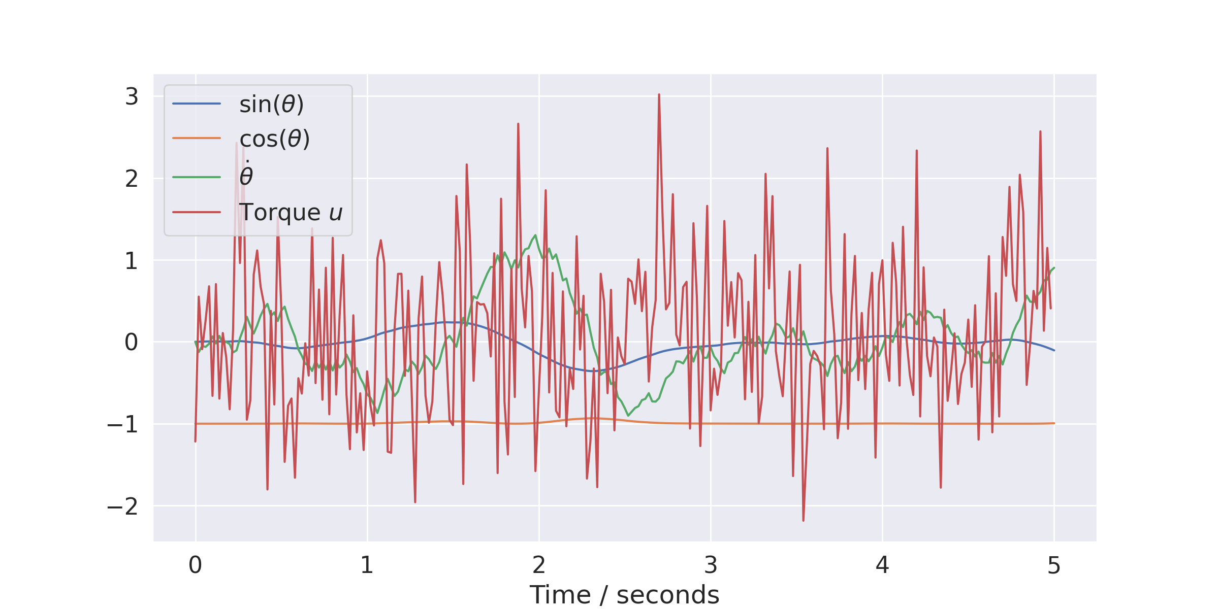
Visualizing trajectories

It is easy to visualize trajectories (i.e., the states \(x_k\) and actions \(u_k\)) during an episode. The following example shows are very bare-boned approach using the irlc.ex01.agent.Agent:

import matplotlib.pyplot as plt
import numpy as np
from irlc import Agent, train
from irlc.ex04.model_pendulum import GymSinCosPendulumEnvironment
env = GymSinCosPendulumEnvironment()

stats, trajectories = train(env, Agent(env), num_episodes=1, return_trajectory=True)

plt.plot(trajectories[0].time, trajectories[0].state[:,0], label="$\\sin(\\theta)$")
plt.plot(trajectories[0].time, trajectories[0].state[:,1], label="$\\cos(\\theta)$")

(Source code, png, hires.png, pdf)

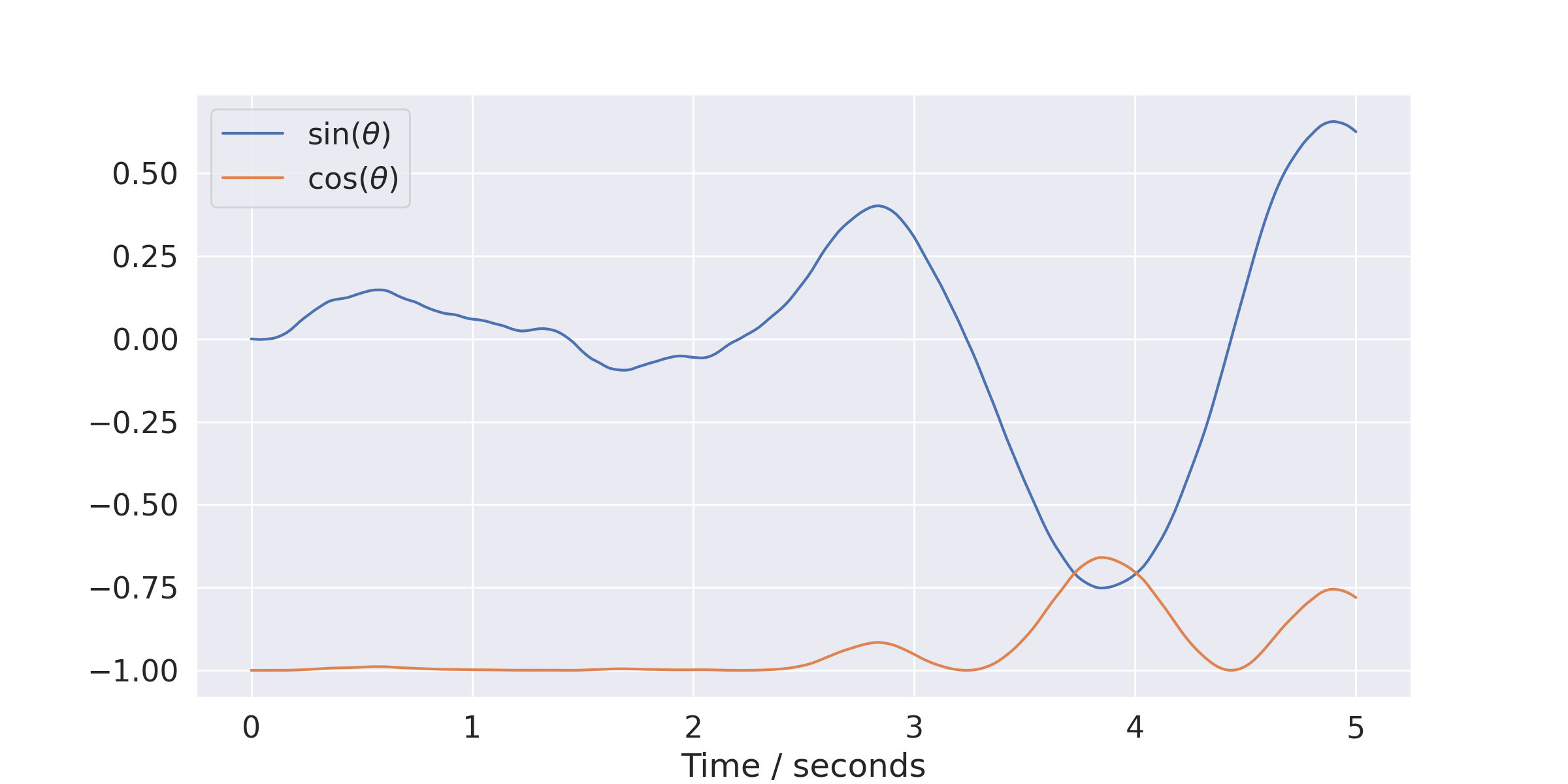
We can simplify this, and get a slightly nicer plot in the process, by using the plot_trajectory() function. It will plot all the coordinates, and you can set the labels in the environment class. The plot shows that the random actions will tend to cancel out, and the system moves very little.

import matplotlib.pyplot as plt
import numpy as np
from irlc import Agent, plot_trajectory, train
from irlc.ex04.model_pendulum import GymSinCosPendulumEnvironment
env = GymSinCosPendulumEnvironment()
stats, trajectories = train(env, Agent(env), num_episodes=1, return_trajectory=True)

plot_trajectory(trajectories[0], env)

(Source code, png, hires.png, pdf)

Tip

The plot_trajectory function extracts the labels from the environment which gets them from the model. You can see how they are defined in GymSinCosPendulumModel.

If you only want to plot a subset of the state or action coordinates you can specify this as extra arguments.

Classes and functions

class irlc.ex04.discrete_control_model.DiscreteControlModel(model, dt, cost=None, discretization_method=None)

A discretized model. To create a model of this type, first specify a symbolic model, then pass it along to the constructor. Since the symbolic model will specify the dynamics as a symbolic function, the discretized model can automatically discretize it and create functions for computing derivatives.

The class will also discretize the cost. Note that it is possible to specify coordinate transformations.

__init__(model, dt, cost=None, discretization_method=None)

Create the discretized model.

Parameters:

• model (ControlModel) – The continuous-time model to discretize.

• dt (float) – Discretization timestep \(\Delta\)

• cost – If this parameter is not specified, the cost will be derived (discretized) automatically from model

• discretization_method – Can be either 'Euler' (default) or 'ei' (exponential integration). The later will assume that the model is a linear.

discretization_method

Initialize symbolic variables representing inputs and actions.

action_labels = None

This field represents the ContinuousSymbolicModel the discrete model is derived from.

property state_size

The dimension of the state vector \(x\), i.e. \(n\) :return: Dimension of the state vector \(n\)

property action_size

The dimension of the action vector \(u\), i.e. \(d\) :return: Dimension of the action vector \(d\)

f(x, u, k=0)

This function implements the dynamics \(f_k(x_k, u_k)\) of the model. They can be evaluated as:

>>> from irlc.ex04.model_pendulum import DiscreteSinCosPendulumModel
>>> model = DiscreteSinCosPendulumModel()
>>> x = [0, 1, 0.4]
>>> u = [1]
>>> print(model.f(x,u) )           # Computes x_{k+1} = f_k(x_k, u_k)
[0.00799991 0.999968   0.51423912]

The model will by default be Euler discretized:

\[x_{k+1} = f_k(x_k, u_k) = x_k + \Delta f(x_k, u_k)\]

except LinearQuadraticModel which will be discretized using Exponential Integration by default.

Parameters:

• x – The state as a numpy array

• u – The action as a numpy array

• k – The time step as an integer (currently this has no effect)

Returns:

The next state \(x_{x+1}\) as a numpy array.

f_jacobian(x, u, k=0)

Compute the Jacobians of the discretized dynamics.

The function will compute the two Jacobian derives of the discrete dynamics \(f_k\) with respect to \(x\) and \(u\):

\[J_x f_k(x,u), \quad J_u f_k(x, u)\]

>>> from irlc.ex04.model_pendulum import DiscreteSinCosPendulumModel
>>> model = DiscreteSinCosPendulumModel()
>>> x = [0, 1, 0.4]
>>> u = [0]
>>> f, Jx, Ju = model.f(x,u)
>>> Jx, Ju = model.f_jacobian(x,u)
>>> print("Jacobian Jx is\\n", Jx)
Jacobian Jx is\n [[ 9.99968000e-01  0.00000000e+00  1.99993600e-02]
 [-7.99991467e-03  0.00000000e+00 -1.59998293e-04]
 [ 1.96400000e-01 -0.00000000e+00  1.00000000e+00]]
>>> print("Jacobian Ju is\\n", Ju)
Jacobian Ju is\n [[0.  ]
 [0.  ]
 [0.15]]

Parameters:

• x – The state as a numpy array

• u – The action as a numpy array

• k – The time step as an integer (currently this has no effect)

Returns:

The two Jacobians computed wrt. \(x\) and \(u\).

class irlc.ex04.control_environment.ControlEnvironment(discrete_model, Tmax=None, supersample_trajectory=False, render_mode=None)

Helper class to convert a discretized model into an environment. See the __init__ function for how to create a new environment using this class. Once an environment has been created, you can use it as any other gym environment:

>>> from irlc.ex04.model_pendulum import GymSinCosPendulumEnvironment
>>> env = GymSinCosPendulumEnvironment(Tmax=4) # Specify we want it to run for a maximum of 4 seconds
>>> env.reset() # Reset both the time and state variable
(array([-8.742278e-08, -1.000000e+00,  0.000000e+00], dtype=float32), {'time_seconds': 0})
>>> u = env.action_space.sample()
>>> next_state, cost, done, truncated, info = env.step(u)
>>> print("Current state: ", env.state)
Current state:  [ 4.46240907e-04 -9.99999900e-01 -4.46245789e-02]
>>> print("Current time", env.time)
Current time 0.02

In this example, tell the environment to terminate after 4 seconds using Tmax (after which done=True)

Note

The step-method will use the (nearly exact) RK4 method to integrate the enviorent over a timespan of dt, and not use the approximate model.f(x_k,u_k, k)-method in the discrete environment which is based on Euler discretization. This is the correct behavior since we want the environment to reflect what happens in the real world and not our apprixmation method.

__init__(discrete_model, Tmax=None, supersample_trajectory=False, render_mode=None)

Creates a new instance. You should use this in conjunction with a discrete model to build a new class. An example:

>>> from irlc.ex04.model_pendulum import DiscreteSinCosPendulumModel
>>> from irlc.ex04.control_environment import ControlEnvironment
>>> from gymnasium.spaces import Box
>>> import numpy as np
>>> class MyGymSinCosEnvironment(ControlEnvironment):
...     def __init__(self, Tmax=5):
...         discrete_model = DiscreteSinCosPendulumModel()
...         self.action_space = Box(low=-np.inf, high=np.inf, shape=(1,), dtype=np.float64)
...         self.observation_space = Box(low=-np.inf, high=np.inf, shape=(3,), dtype=np.float64)
...         super().__init__(discrete_model, Tmax=Tmax)
... 
>>> env = MyGymSinCosEnvironment()
>>> env.reset()
(array([-8.742278e-08, -1.000000e+00,  0.000000e+00], dtype=float32), {'time_seconds': 0})
>>> env.step(env.action_space.sample())
(array([-5.85409543e-04, -9.99999829e-01,  5.85066994e-02]), -83.41189187087281, False, False, {'dt': 0.02, 'time_seconds': 0.02})

Parameters:

• discrete_model (DiscreteControlModel) – The discrete model the environment is based on

• Tmax – Time in seconds until the environment terminates (step returns done=True)

• supersample_trajectory – Used to create nicer (smooth) trajectories. Don’t worry about it.

• render_mode – If human the environment will be rendered (inherited from Env)

step(u)

This works similar to the gym Env.step-function. u is an action in the action-space, and the environment will then assume we (constantly) apply the action u from the current time step, \(t_k\), until the next time step \(t_{k+1} = t_k + \Delta\), where \(\Delta\) is equal to env.model.dt.

During this period, the next state is computed using the relatively exact RK4 simulation, and the incurred cost will be computed using Riemann integration.

\[\int_{t_k}^{t_k+\Delta} c(x(t), u(t)) dt\]

Note

The gym environment requires that we return a cost. The reward will therefore be equal to minus the (integral) of the cost function.

In case the environment terminates, the reward will include the terminal cost. \(c_F\).

Parameters:

u – The action we apply \(u\)

Returns:

• state - the state we arrive in

• reward - (minus) the total (integrated) cost incurred in this time period.

• done - True if the environment has finished, i.e. we reached env.Tmax.

• truncated - True if the environment was forced to terminated prematurely. Assume it is False and ignore it.

• info - A dictionary of potential extra information. Includes info['time_seconds'], which is the current time after the step function has completed.

reset()

Reset the environment to the initial state. This will by default be the value computed using `self.discrete_model.reset()`.

Returns:

• state - The initial state the environment has been reset to

• info - A dictionary with extra information, in this case that time begins at 0 seconds.

render()

Compute the render frames as specified by render_mode during the initialization of the environment.

The environment’s metadata render modes (env.metadata[“render_modes”]) should contain the possible ways to implement the render modes. In addition, list versions for most render modes is achieved through gymnasium.make which automatically applies a wrapper to collect rendered frames.

Note:

As the render_mode is known during __init__, the objects used to render the environment state should be initialised in __init__.

By convention, if the render_mode is:

• None (default): no render is computed.

• “human”: The environment is continuously rendered in the current display or terminal, usually for human consumption. This rendering should occur during step() and render() doesn’t need to be called. Returns None.

• “rgb_array”: Return a single frame representing the current state of the environment. A frame is a np.ndarray with shape (x, y, 3) representing RGB values for an x-by-y pixel image.

• “ansi”: Return a strings (str) or StringIO.StringIO containing a terminal-style text representation for each time step. The text can include newlines and ANSI escape sequences (e.g. for colors).

• “rgb_array_list” and “ansi_list”: List based version of render modes are possible (except Human) through the wrapper, gymnasium.wrappers.RenderCollection that is automatically applied during gymnasium.make(..., render_mode="rgb_array_list"). The frames collected are popped after render() is called or reset().

Note:

Make sure that your class’s metadata "render_modes" key includes the list of supported modes.

Changed in version 0.25.0: The render function was changed to no longer accept parameters, rather these parameters should be specified in the environment initialised, i.e., gymnasium.make("CartPole-v1", render_mode="human")

close()

After the user has finished using the environment, close contains the code necessary to “clean up” the environment.

This is critical for closing rendering windows, database or HTTP connections. Calling close on an already closed environment has no effect and won’t raise an error.

class irlc.ex04.discrete_control_cost.DiscreteQRCost(Q, R, H=None, q=None, r=None, qc=0, QN=None, qN=None, qcN=0)

This class represents the cost function for a discrete-time model. In the simulations, we are going to assume that the cost function takes the form:

\[\sum_{k=0}^{N-1} c_k(x_k, u_k) + c_N(x_N)\]

And this class will specifically implement the two functions \(c\) and \(c_N\). They will be assumed to have the quadratic form:

\[\begin{split}c_k(x_k, u_k) & = \frac{1}{2} x_k^T Q x_k + \frac{1}{2} u_k^T R u_k + u^T_k H x_k + q^T x_k + r^T u_k + q_0, \\ c_N(x_N) & = \frac{1}{2} x_N^T Q_N x_N + q_N^T x_N + q_{0,N}.\end{split}\]

So what all of this boils down to is that the class just need to store a bunch of matrices and vectors.

You can add and scale cost-functions

A slightly smart thing about the cost functions are that you can add and scale them. The following provides an example:

>>> from irlc.ex04.discrete_control_cost import DiscreteQRCost
>>> import numpy as np
>>> cost1 = DiscreteQRCost(np.eye(2), np.zeros(1) ) # Set Q = I, R = 0
>>> cost2 = DiscreteQRCost(np.ones((2,2)), np.zeros(1) ) # Set Q = 2x2 matrices of 1's, R = 0
>>> print(cost1.Q) # Will be the identity matrix.
[[1. 0.]
 [0. 1.]]
>>> cost = cost1 * 3 +  cost2 * 2
>>> print(cost.Q) # Will be 3 x I + 2
[[5. 2.]
 [2. 5.]]

__init__(Q, R, H=None, q=None, r=None, qc=0, QN=None, qN=None, qcN=0)

c(x, u, k=None, compute_gradients=False)

Evaluate the (instantaneous) part of the function \(c_k(x_k,u_k)\). An example:

>>> from irlc.ex04.discrete_control_cost import DiscreteQRCost
>>> import numpy as np
>>> cost = DiscreteQRCost(np.eye(2), np.eye(1)) # Set Q = I, R = 0
>>> cost.c(x = np.asarray([1,2]), u=np.asarray([0]), compute_gradients=False) # should return 0.5 * x^T Q x = 0.5 * (1 + 4)
2.5

The function can also return the derivates of the cost function if compute_derivates=True

Parameters:

• x – The state \(x_k\)

• u – The action \(u_k\)

• k – The time step \(k\) (this will be ignored)

• compute_gradients – if True the function will compute gradients and Hessians.

Returns:

• c - The cost as a float

• c_x - The derivative with respect to \(x\)

cN(x, compute_gradients=False)

Evaluate the terminal (constant) term in the cost function \(c_N(x_N)\). An example:

>>> from irlc.ex04.discrete_control_cost import DiscreteQRCost
>>> import numpy as np
>>> cost = DiscreteQRCost(np.eye(2), np.zeros(1), QN=np.eye(2)) # Set Q = I, R = 0
>>> c, Jx, Jxx = cost.cN(x=2*np.ones((2,)), compute_gradients=True)
>>> c # should return 0.5 * x_N^T * x_N = 0.5 * 8
4.0

Parameters:

• x – Terminal state \(x_N\)

• compute_gradients – if True the function will compute gradients and Hessians of the cost function.

Returns:

The last (terminal) part of the cost-function \(c_N\)

classmethod zero(state_size, action_size)

Creates an all-zero cost function, i.e. all terms \(Q\), \(R\) are set to zero.

>>> from irlc.ex04.discrete_control_cost import DiscreteQRCost
>>> cost = DiscreteQRCost.zero(2, 1)
>>> cost.Q # 2x2 zero matrix
array([[0., 0.],
       [0., 0.]])
>>> cost.R # 1x1 zero matrix.
array([[0.]])

Parameters:

• state_size – Dimension of the state vector \(n\)

• action_size – Dimension of the action vector \(d\)

Returns:

A DiscreteQRCost with all zero terms.

goal_seeking_terminal_cost(xN_target, QN=None)

Create a discrete cost function which is minimal when the final state \(x_N\) is equal to a goal state \(x_N^*\). Concretely, it will return a cost function of the form

\[c_N(x_N) = \frac{1}{2} (x^*_N - x_N)^\top Q (x^*_N - x_N)\]

>>> from irlc.ex04.discrete_control_cost import DiscreteQRCost
>>> import numpy as np
>>> cost = DiscreteQRCost.zero(2, 1)
>>> cost += cost.goal_seeking_terminal_cost(xN_target=np.ones((2,)))
>>> print(cost.qN)
[-1. -1.]
>>> print(cost)
Discrete-time cost function:
> Non-zero terms in c_N(x_N):
 * QN = 
[[1. 0.]
 [0. 1.]]
 * qN = [-1. -1.]
 * qcN = 1.0

Parameters:

• xN_target – Target state \(x_N^*\)

• Q – Cost matrix \(Q\)

Returns:

A DiscreteQRCost object corresponding to the goal-seeking cost function

goal_seeking_cost(x_target, Q=None)

Create a discrete cost function which is minimal when the state \(x_k\) is equal to a goal state \(x_k^*\). Concretely, it will return a cost function of the form

\[c_k(x_k, u_k) = \frac{1}{2} (x^*_k - x_k)^\top Q (x^*_k - x_k)\]

>>> from irlc.ex04.discrete_control_cost import DiscreteQRCost
>>> import numpy as np
>>> cost = DiscreteQRCost.zero(2, 1)
>>> cost += cost.goal_seeking_cost(x_target=np.ones((2,)))
>>> print(cost.q)
[-1. -1.]
>>> print(cost)
Discrete-time cost function:
> Non-zero terms in c_k(x_k, u_k):
 * Q = 
[[1. 0.]
 [0. 1.]]
 * q = [-1. -1.]
 * qc = 1.0

Parameters:

• x_target – Target state \(x_k^*\)

• Q – Cost matrix \(Q\)

Returns:

A DiscreteQRCost object corresponding to the goal-seeking cost function

irlc.utils.irlc_plot.plot_trajectory(trajectory, env=None, xkeys=None, ukeys=None)

Used to visualize trajectories returned from the train()-function. An example:

import matplotlib.pyplot as plt
import numpy as np
from irlc import Agent, plot_trajectory, train
from irlc.ex04.model_pendulum import GymSinCosPendulumEnvironment
env = GymSinCosPendulumEnvironment()
stats, trajectories = train(env, Agent(env), num_episodes=1, return_trajectory=True)
plot_trajectory(trajectories[0], env)

(Source code, png, hires.png, pdf)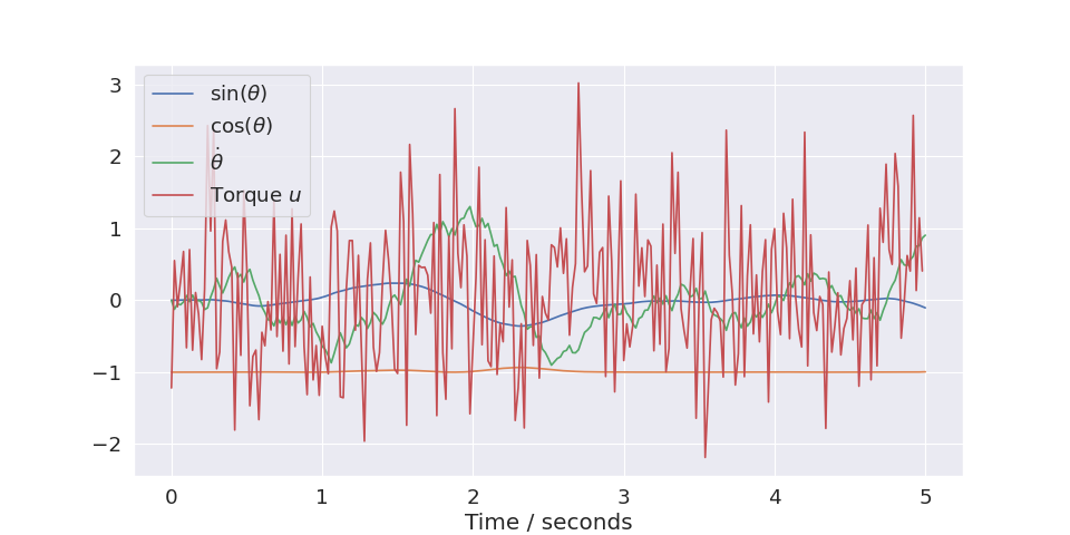

Labels will be derived from the env if supplied. The parameters xkeys and ukeys can be used to limit which coordinates are plotted. For instance, if you only want to plot the first two x-coordinates you can set xkeys=[0,1]:

(Source code, png, hires.png, pdf)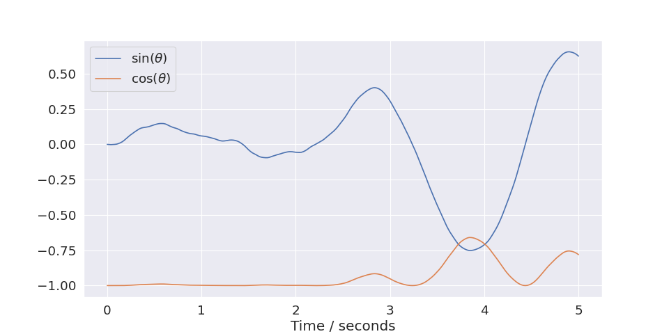

Parameters:

• trajectory – A single trajectory computed using train (see example above)

• env – A gym control environment (optional)

• xkeys – List of integers corresponding to the coordinates of \(x\) we wish to plot

• ukeys – List of integers corresponding to the coordinates of \(u\) we wish to plot

Tip

If the plot does not show, you might want to import matplotlib as import matplotlib.pyplot as plt and call plt.show()

Solutions to selected exercises

Solution to problem 1

Part a: At time \(\Delta\) the angle is \(w(\Delta) = 0\) because it is the first coordinate of \(\mathbf x_1\):

\[\begin{split}\mathbf x_1 = \mathbf x_0 + \Delta f(\mathbf x_0, 0) = \begin{bmatrix} 0 \\ \Delta \end{bmatrix}\end{split}\]

Part b: We just do one more Euler update to get:

\[\begin{split}\mathbf x_2 = \mathbf x_1 + \Delta f(\mathbf x_1, 0) = \Delta \begin{bmatrix} \Delta \\ 1 + \cos( 0 ) \end{bmatrix}\end{split}\]

So the answer is \(w(2\Delta) = \Delta^2\).

Part c: Similar to the part a we get:

\[\begin{split}\mathbf x_1 & = \mathbf x_0 + \Delta f(\mathbf x_0, u_0) \\ & = \begin{bmatrix} \frac{\pi}{2} \\ 0 \end{bmatrix} + \Delta \begin{bmatrix} 0 \\ \cos(u_0 + \frac{\pi}{2} ) \end{bmatrix} \\ & = \begin{bmatrix} \frac{\pi}{2} \\ -\Delta \sin(u_0) \end{bmatrix}\end{split}\]

So the answer is \(w(\Delta) = \frac{\pi}{2}\). This means that regardless of how much force we apply to the system, Euler discretization predict the system does not change position during the first \(\Delta\) time interval – which is obviously not true. The bottom line is that Euler discretization is not accurate unless \(\Delta\) is much smaller than the time interval we wish to simulate the system over.

Solution to problem 2: PID

The answer is c.

At the very first time step, the angle is \(x = 6\), the control output is \(u=-6\), and the target is \(x^* = 4\). This means that the control output satisfy: \(u = K_p (x^* - x) = -2K_p\). Solving we get \(K_p = 3\).

Problem 4.1 and 4.2: Discretization

Problem 4.3: PID

Problem 4.4: PID Agent

Problem 4.5 and 4.6: Pendulum balancer