Exercise 7: Exploration and Bandits#
Note
This page contains background information which may be useful in future exercises or projects. You can download this weeks exercise instructions from here:
Slides: [1x] ([6x]). Reading: Chapter 1; Chapter 2-2.7; 2.9-2.10, [SB18].
You are encouraged to prepare the homework problems 1 (indicated by a hand in the PDF file) at home and present your solution during the exercise session.
To get the newest version of the course material, please see Making sure your files are up to date
Bandits#
Bandits are an example of a particular, simplified reinforcement learning setup where the emphasis is on exploration.
We are therefore going to model bandits as reinforcement learning problems using the Env and Agent.
Let’s first explore the bandit problem corresponding to the simple 10-armed bandit in (Sutton and Barto [SB18]). Recall that this bandit:
There are \(k=10\) arms.
An action \(a_k \in \{0, 1, .., 9\}\) selects an arm, and we then obtain a reward \(r_t\)
An episode corresponds to e.g. \(T=1000\) such interactions. The purpose is to maximize the accumulated reward
We want to be able to reset the environment and re-do the experiment many times
A basic interaction with the environment is as follows:
>>> from irlc.ex07.bandits import StationaryBandit
>>> env = StationaryBandit(k=10)                    # 10-armed testbed.
>>> env.reset()                                     # Reset env.q_star
(0, {})
>>> s, r, _, _, info = env.step(3)
>>> print(f"The reward we got from taking arm a=3 was {r=}")
The reward we got from taking arm a=3 was r=np.float64(0.04640427343592121)
The script print out the immediate reward in the first step \(r_0\).
Internally, the environment will store the (expected) reward for each arm as env.q_star. These values are reset (sampled from a normal distribution)
when the irlc.ex07.bandits.StationaryBandit.reset() method is called, and can be used to compute the average regret. An example:
>>> from irlc.ex07.bandits import StationaryBandit
>>> env = StationaryBandit(k=4)     # 4-armed testbed.
>>> env.reset()                     # Reset all parameters.
(0, {})
>>> env.q_star
array([-0.13778623, -0.14346716, -0.43211553, -1.48196392])
>>> env.reset()                     # Reset again
(0, {})
>>> env.q_star
array([-0.99634987,  1.03495783, -0.23327224,  2.04833132])
>>> env.optimal_action              # This variable stores the optimal action
np.int64(3)
>>> _, r, _, _, info = env.step(2)  # Take action a=2
>>> print(f"Reward from a=2 was {r=}, the gab was {info['gab']=}")
Reward from a=2 was r=np.float64(2.145184696023021), the gab was info['gab']=np.float64(2.2816035611772456)
This code also computes the per-step gab \(Delta\), info['gab'], which for an action \(a\) is defined as
Perhaps you can tell how it can be computed using env.optimal_action and env.q_star?
Implementing a bandit environment#
To implement a new bandit environment, all you need to do is to implement the
reward function and compute the gab. To simplify things I have made a helper class
BanditEnvironment where you only need to implement the reset() function and a function
bandit_step() which accepts an action and returns the reward \(r_t\) and gab.
# bandits.py
class StationaryBandit(BanditEnvironment):
    def reset(self):
        """ Set q^*_k = N(0,1) + mean_value. The mean_value is 0 in most examples. I.e., implement the 10-armed testbed environment. """
        self.q_star = np.random.randn(self.k) + self.q_star_mean
        self.optimal_action = np.argmax(self.q_star) # Optimal action is the one with the largest q^*-value.
    def bandit_step(self, a):
        # Actual logic goes here. Use self.q_star[a] to get mean reward and np.random.randn() to generate random numbers.
        return reward, gab
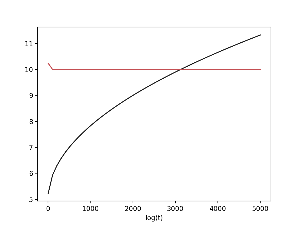
Training and visualizing bandit agents#
Agents for bandits problems are implemented as usual by overwritign the pi() and train function in the Agent class.
You can train the bandit agent by using the train() as usual, but to simplify things I have made a convenience method to train and visualize multiple bandits as follows:
Tip
If you set use_cache=True then old simulations will be stored and plotted until there are
max_episodes total simulations. Saving old simulations for later plotting is essential in reinforcement learning.
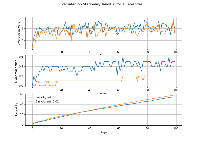
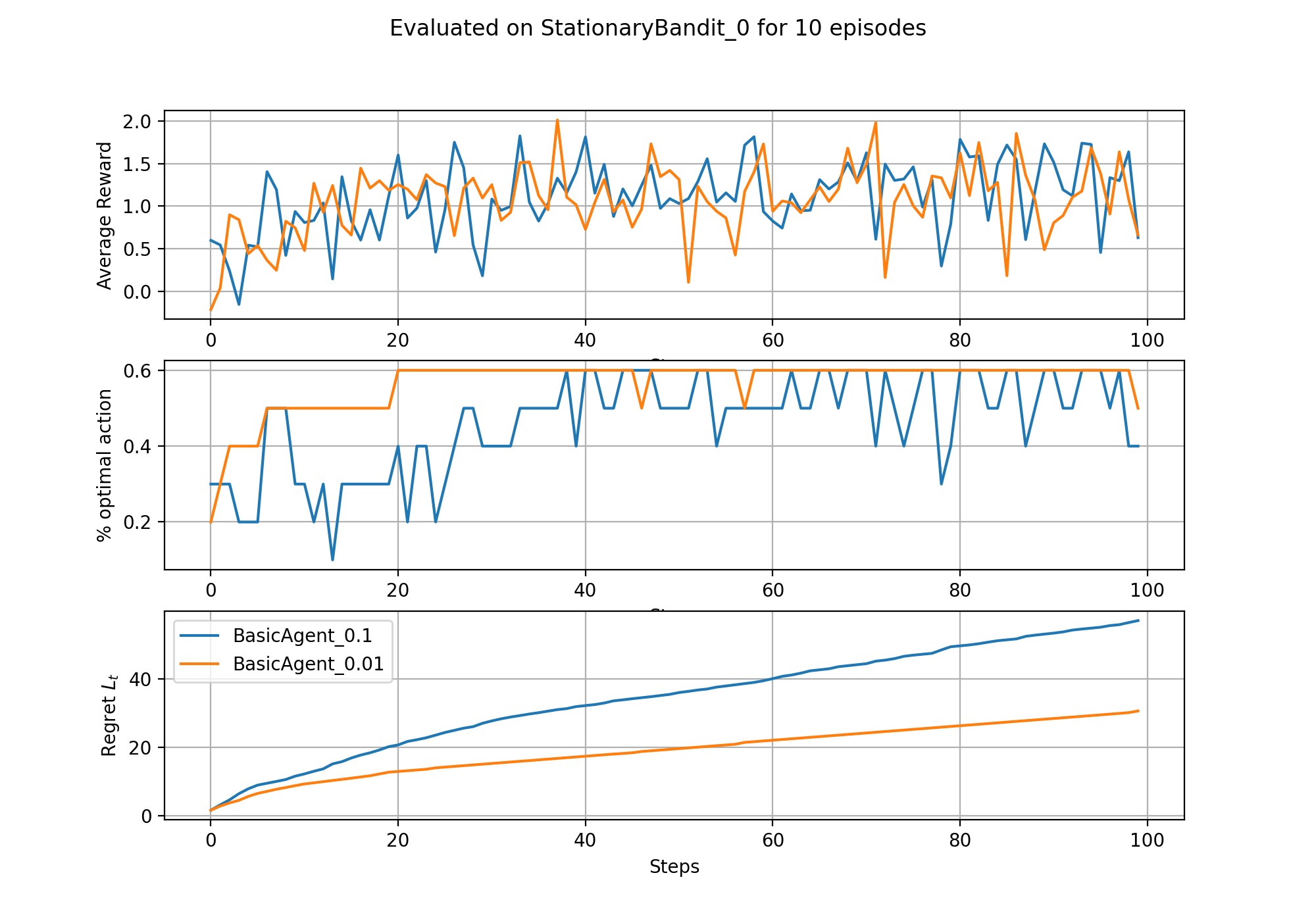
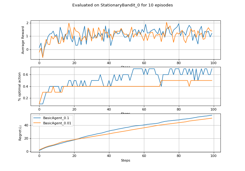
>>> from irlc.ex07.bandits import StationaryBandit, eval_and_plot
>>> from irlc.ex07.simple_agents import BasicAgent
>>> env = StationaryBandit(k=10)                                                                # 10-armed testbed
>>> agents = [BasicAgent(env, epsilon=.1), BasicAgent(env, epsilon=.01)]                        # Create two agents
>>> k = eval_and_plot(env, agents, num_episodes=10, steps=100, max_episodes=10, use_cache=True)    # Fight!
(Source code, png, hires.png, pdf)
Classes and functions#
- class irlc.ex07.bandits.BanditEnvironment(k)[source]#
Bases:
EnvA helper class for defining bandit problems similar to e.g. the 10-armed testbed discsused in (SB18). We are going to implement the bandit problems as greatly simplfied gym environments, as this will allow us to implement the bandit agents as the familiar
Agent. I hope this way of doing it will make it clearer that bandits are in fact a sort of reinforcement learning method.The following code shows an example of how to use a bandit environment:
>>> from irlc.ex07.bandits import StationaryBandit
>>> env = StationaryBandit(k=10)                    # 10-armed testbed.
>>> env.reset()                                     # Reset env.q_star
(0, {})
>>> s, r, _, _, info = env.step(3)
>>> print(f"The reward we got from taking arm a=3 was {r=}")
The reward we got from taking arm a=3 was r=np.float64(-2.562378734357159)
- __init__(k)[source]#
Initialize a bandit problem. The observation space is given a dummy value since bandit problems of the sort (SB18) discuss don’t have observations.
- Parameters:
k (
int) – The number of arms.
- reset()[source]#
Use this function to reset the all internal parameters of the environment and get ready for a new episode. In the (SB18) 10-armed bandit testbed, this would involve resetting the expected return
\[q^*_a\]The function must return a dummy state and info dictionary to agree with the gym
Envclass, but their values are irrelevant- Returns:
s - a state, for instance 0
info - the info dictionary, for instance {}
- bandit_step(a)[source]#
This helper function simplify the definition of the environments
step-function.Given an action \(r\), this function computes the reward obtained by taking that action \(r_t\) and the gab. This is defined as the expected reward we miss out on by taking the potentially suboptimal action \(a\) and is defined as:
\[\Delta = \max_{a'} q^*_{a'} - q_a\]Once implemented, the reward and regret enters into the
stepfunction as follows:>>> from irlc.ex07.bandits import StationaryBandit >>> env = StationaryBandit(k=4) # 4-armed testbed. >>> env.reset() # Reset all parameters. (0, {}) >>> _, r, _, _, info = env.step(2) # Take action a=2 >>> print(f"Reward from a=2 was {r=}, the gab was {info['gab']=}") Reward from a=2 was r=np.float64(0.7547085011448744), the gab was info['gab']=np.float64(2.597446898095079)
- Parameters:
a – The current action we take
- Returns:
r - The reward we thereby incur
gab - The regret gab \(\Delta\) incurred by taking this action (0 for an optimal action)
- step(action)[source]#
You do not have to edit this function. In a bandit environment, the step function is simplified greatly since there are no states to keep track on. It should simply return the reward incurred by the action
aand (for convenience) also returns the gab in theinfo-dictionary.- Parameters:
action – The current action we take \(a_t\)
- Returns:
next_state - This is always
Nonereward - The reward obtained by taking the given action. In (SB18) this is defined as \(r_t\)
terminated - Always
False. Bandit problems don’t terminate.truncated - Always
Falseinfo - For convenience, this includes the gab (used by the plotting methods)
- class irlc.ex07.bandits.StationaryBandit(k, q_star_mean=0)[source]#
Bases:
BanditEnvironmentImplement the ‘stationary bandit environment’ which is described in (SB18, Section 2.3) and used as a running example throughout the chapter.
We will implement a version with a constant mean offset (q_star_mean), so that
q* = x + q_star_mean, x ~ Normal(0,1)
q_star_mean can just be considered to be zero at first.
- __init__(k, q_star_mean=0)[source]#
Initialize a bandit problem. The observation space is given a dummy value since bandit problems of the sort (SB18) discuss don’t have observations.
- Parameters:
k – The number of arms.
- reset()[source]#
Set q^*_k = N(0,1) + mean_value. The mean_value is 0 in most examples. I.e., implement the 10-armed testbed environment.
- bandit_step(a)[source]#
Return the reward/gab for action a for the simple bandit. Use self.q_star (see reset-function above). To implement it, implement the reward (see the description of the 10-armed testbed for more information. How is it computed from q^*_k?) and also compute the gab.
As a small hint, since we are computing the gab, it will in fact be the difference between the value of q^* corresponding to the current arm, and the q^* value for the optimal arm. Remember it is 0 if the optimal action is selected.
Solutions to selected exercises#
Solution to the conceptual problem 1
Part a: Since the simple bandit explore at random, we can never rule out that it explored, because it might select the optimal action during exploration.
However, if the agent selects a sub-optimal action, we know it must have occured by exploration. We track the Q-values:
$t=1$: \(Q(1)=-1\), \(Q(2)=0\), \(Q(3)=0\), \(Q(4)=0\)
$t=2$: \(Q(1)=-1\), \(Q(2)=1\), \(Q(3)=0\), \(Q(4)=0\)
$t=3$: \(Q(1)=-1\), \(Q(2)=\frac{-1}{2}\), \(Q(3)=0\), \(Q(4)=0\)
$t=4$: \(Q(1)=-1\), \(Q(2)=\frac{1}{3}\), \(Q(3)=0\), \(Q(4)=0\)
$t=5$: \(Q(1)=-1\), \(Q(2)=\frac{1}{3}\), \(Q(3)=0\), \(Q(4)=0\)
So we see the method must have selected a sub-optimal action at time \(t=4`and at time :math:`t=5\).
Part b+c: Based on the figure, the average regret of the first three arms is the horizontal black line so about 0.1, -0.8 and 1.5. The best arm is \(a=3\) since it has the highest average regret of all ten arms and therefore the regret is
\(1.5 - 0.1 = 1.4\)
\(1.5 - (-0.8) = 2.3\)
\(1.5 - 1.5 = 0\)
Note that the regret can never be negative. It is called regret because is the average reward we miss out on. Therefore, we have no regret when we take the optimal arm, and more regret the worse the arm is compared to the optimal.
Problem 8.1
Problem 8.2
Conceptual Question: UCB Bandits
Part a: Since the rewards are always the same the \(Q\)-values are just the average of the same number and therefore a constant. So:
Part b: UCB1 will select arm 1 as it has the highest bound (see above). This is natural, sicne it has a higher reward estimate, and we have tried them the same amount of time and therefore there is no reason one should be preferred over the other due to exploration.
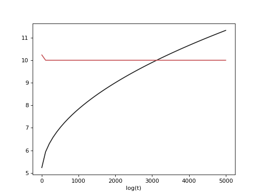
Part c: For \(t \geq 1000\) will be:
Part d: The ‘rough sketch’ indicate that the upper confidence bound grows for \(f_0\) (logarithmically) and fall for \(f_1\) (roghly as \(\frac{1}{t}\)) towards 10. The curve for \(f_0\) starts out 5 units below \(f_1\) and so they cross… eventually.. long after the heat death of the universe:
(Source code, png, hires.png, pdf)
Cheat mode on#
Part e: When they cross, the algorithm will change arm.